Why Relational Databases are better than spreadsheets
Running notebook: Investigation progress
- Getting hold of the data
- Using a tool discovered on GitHub
In the previous chapter, we installed and configured GarminDB to
retrieve our Garmin data. The program has since done its job and
organised everything into five SQLite database files (.db), ready for
analysis.
Before we start extracting information from them, it is key to understand what this format is, what it means for the data, and why I am very happy the developers of GarminDB chose it.
In particular, I will introduce the advantages relational databases offer for storing and analysing this type of data that spreadsheets don’t. This chapter may be a bit more conceptual than usual, but I’ll do my best to keep everything as grounded as possible.
As for the running itself, things are progressing nicely. My training programme is now entering its fourth week, and seven runs have already been entered into our newly created database. Tomorrow I even have a 2-mile time trial scheduled. We shall soon have enough data to start looking at some of these data.
Why not just a giant spreadsheet?
At first glance, a spreadsheet may seem like a simpler choice. Most people are familiar with Excel or Google Sheets, and for small datasets, they are often perfectly adequate.
But the problem is that Garmin records many different types of data. Activities have distances, durations and routes. Daily summaries include steps, calories and floors climbed. Sleep has its own measurements. Heart rate is recorded at regular intervals throughout the day. Body weight changes much less frequently.
These data do not naturally fit into the same table. If we tried to force everything into a single spreadsheet, we would quickly run into a choice between two undesirable options.
The first would be to create hundreds of columns, most of which would be empty for any given row. A heart-rate measurement has no running distance. A run has no sleep stage. A body weight measurement has no GPS coordinates.
The second would be to duplicate information repeatedly. Every heart-rate measurement recorded during a run would need to store the date, activity identifier and other details again and again, making the dataset larger, harder to maintain, and more prone to inconsistencies. And the file would grow so big you couldn’t open it anymore.
Neither solution is particularly appealing. More importantly, neither reflects the way these data are naturally organised.
And that’s why simple spreadsheets usually do not form the backbone of data science with large datasets – although they have some perks like allow for quick access and inspection of the data.
Luckily, there is a better way.
Relational Databases
GarminDB does more than download and unpack Garmin files. It also organises their contents into a relational database with a carefully designed structure.
A relational database stores information across multiple tables rather than forcing everything into a single large dataset. You can think of these tables as spreadsheet tabs, except that they are explicitly connected to one another, with extra constraints that ensure the coherence of the whole. Together, they form a global representation of the data rather than a collection of independent tables.
One table = One type of info
A table describes one clearly defined type of object or event.
In GarminDB, one table stores activities, another the individual laps within those activities, and another the measurements recorded throughout each activity. Each table has its own structure and fields because it answers a different kind of question.
Organising data this way has several advantages. Fields referring to the same information always have the same name and data type. They are also always grouped at the same place, and the information only needs to be stored once, rather than repeated across the database.
For example, the general characteristics of a run (date, distance or
average heart rate) are stored once in activities. The laps associated
with that run simply refer back to it through activity_id, instead of
repeating the same information on every row.
This reduces duplication and prevents inconsistencies. Each piece of information has a single authoritative location.
Tables are connected through a database schema
Separating information into tables would not be particularly useful if those tables could not be connected again.
These connections are defined through shared identifiers. A unique activity identifier was integrated to the activities table and in every table containing information related to that activity (see figure below). This allows retrieving the main characteristics of a run, along with its laps, heart rate records, and other measurements.
The organisation of the tables and the relationships between them form
the database schema, as in this figure.
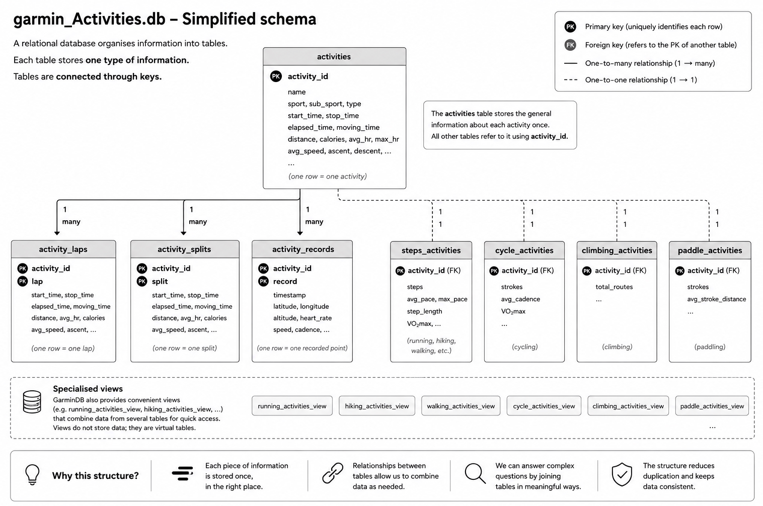
garmin_Activities.db relational
database produced by GarminDB. Each table stores a specific type of
information and is connected to related tables through shared keys. Note: This figure was automatically generated by ChatGPT. It may not represent everything with maximum accuracy, but it is enough to explain the concepts I want to discuss.
From this schema, we can see that the activities table lies at the
top. This table contains all the generic information of the activity
(e.g., sport type, date, name, summary statistics), and all the other
tables contain observations measured during that activity.
The distinction between activities and activity_records illustrates
this well. The table activities stores summary information about each
run, such as its total distance or average speed. The table
activity_records stores the hundreds (or even thousands) of individual
measurements collected during that run, including the speed recorded at
each point in time. The summary is stored once; the measurements are
stored separately.
You can also see the field activity_id is found in every table. It is
the field that links any observation with its activity. So even if the
data are split across several tables, everything remains fully connected
through activity_id.
And the tables have relationships. A one-to-one relationship means
that for each activity_id in activities, there is only one observation
in steps_activities.
In contrast, a one-to-many relationship means that for each activity_id
in activities, there can be many observations in activity_records.
And the latter can be read the opposite way, many-to-one, meaning that
many observations in activity_records can have the same observation in
activities. Importantly, they must have one observation. You cannot
have activity_ids in activity_records without a corresponding entry
in activities
These relationships are one of the greatest strengths of relational databases. They allow the data to be split across multiple tables without losing coherence. Constraints ensure that related observations always point to valid entries in other tables, making inconsistencies much harder to introduce than in ordinary spreadsheets.
In other words, the database itself helps protect the integrity of your data. It is not only a container for information, but also a set of rules describing how that information is allowed to relate.
Spreadsheets do not provide that level of data security.
How to interact with a relational database?
Unlike spreadsheets, relational databases are not usually manipulated directly. Instead, we ask them questions using a language called SQL (Structured Query Language).
Fortunately, understanding SQL is no longer a requirement for data
scientists (altough knowing some basics is always recommended). In R,
packages such as dbplyr allow us to query databases using the
tidyverse syntax while translating our code into SQL behind the
scenes. So you no longer need to learn two (very) different languages to
intarface with your data.
But I won’t say more about this here and eep the suspense intact because we will use this approach in the next chapter to start extracting information from our running database.
Many flavours of relational databases - why is SQLite a good choice here?
Relational databases come in many flavours. Large organisations often
rely on database servers such as PostgreSQL, MySQL, or
Microsoft SQL Server, which are designed to support many users working
simultaneously. These are the solutions that support many online data
platforms.
SQLite takes a different approach. The entire database is stored in a
single file, making it lightweight, portable and easy to distribute.
There is no server to install or administer, making it an excellent
choice for local data analysis projects such as ours.
And for those of you out there that, like me, still like to directly look at the data outside of a programming interface, all you need to do is download an SQLite file viewer (I use DB Browser for SQLite but there are many free options out there). From there, you can navigate your different tables and “see” the raw data.

What’s next
We now understand why GarminDB organised our data into a relational database, how the information is distributed across multiple connected tables, and why this structure is well-suited to data analysis.
Understanding the structure is only the first step. In the next chapter, I will finally start asking questions and extracting my running data from the database. This is where the structure we have just explored will start to pay off.