gbif4crest calibration dataset v3 for CREST

Manuel Chevalier

2025-02-03

What is this this dataset and should I it?

I developed this calibration dataset to enable the use of crestr in many regions for many proxies (See Fig. 1). In previous version, there were also distribution data for insects. I did not include such data in the new calibration dataset because some (palaeo)entomologists mentioned that the large-scale climatologies I used to assign climate values to each grid cell (see below) do not reflect the local environments / microclimates many insects experience.

Should you use this dataset? Only if you want to. You do not have to use it if you have access to appropriate calibration data that have important properties for your analysis. In such cases, I recommend using such data over which you have total control and skipping the gbif4crest calibration data. In addition, CREST can be used with many proxies for which I did not compile data, provided that their spatial distribution can be related to climate parameters to reconstruct.

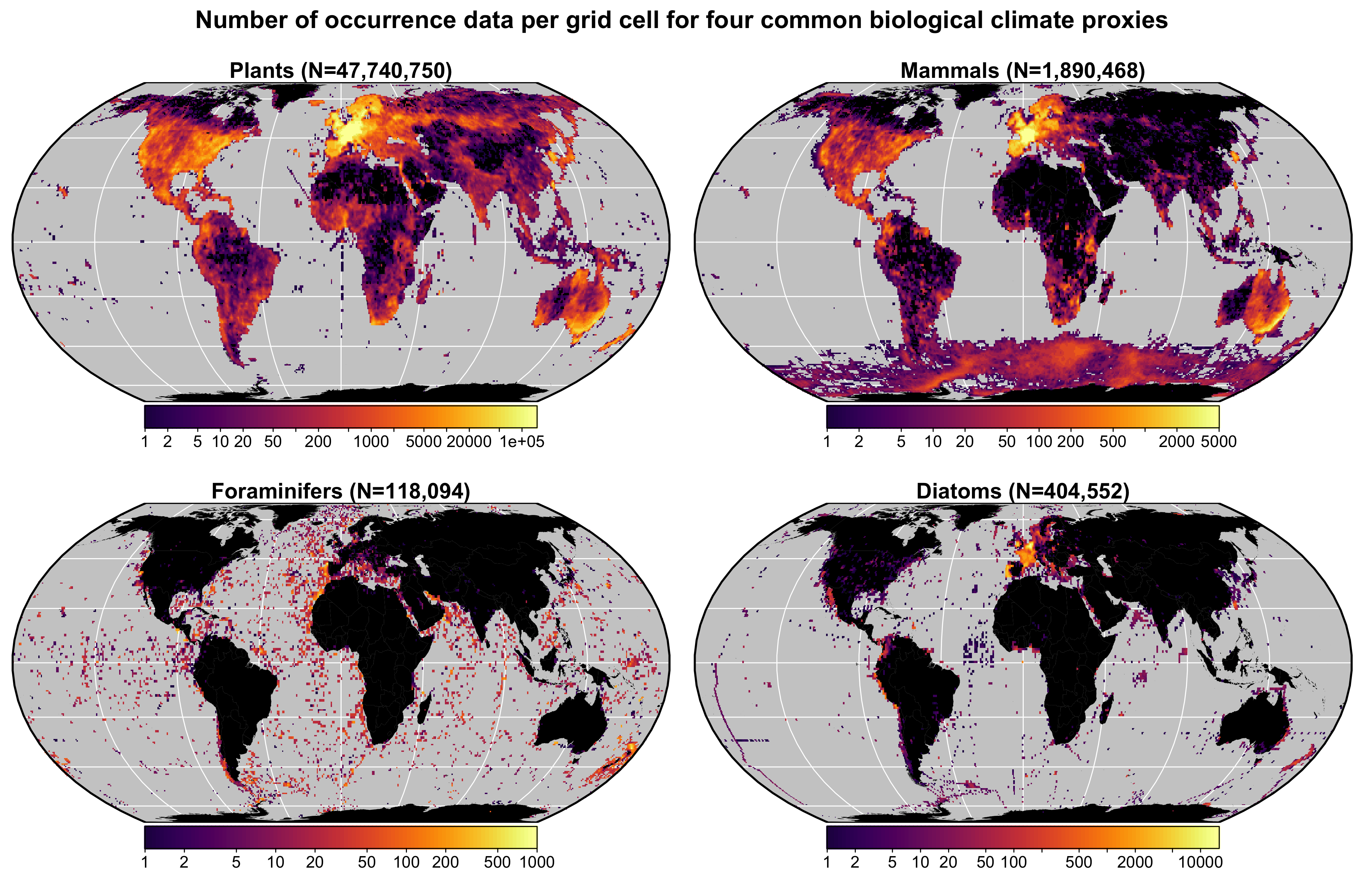
Fig. 1 Data density of the four climate proxies available in the gbif4crest calibration database. The total number of unique species occurrences (N) is indicated for each proxy. The maps are based on the ‘Equal Earth’ map projection to better account for the relative sizes of the different continents.

Source of the calibration data

A multiproxy calibration dataset to estimate PDFs from a global collection of geolocalised presence-only data (hereafter proxy distributions) was first presented in [1]. These data were obtained from the Global Biodiversity Information Facility (GBIF) database, an online collection of geolocalised observations of biological entities [2-10].

The coordinates of all the presence records of these four common palaeoecological fossil proxies were upscaled at a spatial resolution of 1/12° (roughly 0.0833°) and subsequently associated with terrestrial and oceanic environmental variables at the same resolution [11-17] (see details in Table 1). The spatial resolution is an empirical trade-off between numerous factors, including the resolution of the presence data, the quality of the data or the spatial representativity of the studied proxy. However, this tradeoff may be suboptimal in some situations, and may be a reason to consider using another calibration dataset.

In its current version (V3), the gbif4crest calibration dataset contains about 50 million unique presence data for four proxies. Unfortunately, the density of available data varies strongly between proxies and regions (Fig. 1). Plant data dominate the calibration dataset (>47 million unique occurrences) and allow for the use of crestr across all landmasses where vegetation currently grows. For the proxies, the datasets are still incomplete in many regions, restricting the use of crestr (e.g. mammals across most of Asia). However, these datasets are regularly updated by GBIF. For example, the first version of the gbif4crest dataset released in 2018 contained about 17.5 million QDGC entries, the second version about 25.3 and the latest version presented here contains nearly 50 million entries (~300% increase in about 6 years). The range of ‘reconstructible’ areas is thus rapidly broadening (see, for instance, the coverage of Russia by plant data compared to the first version of the gbif4crest dataset [1].

Table 1 List of terrestrial and marine variables available in the gbif4crest database. Each one can be selected in crestr using its associated code. List of abbreviations: (Temp.) Temperature, (Precip.) Precipitation, (SST) Sea Surface Temperature, (SSS) Sea Surface Salinity.

Code	Full name	Source
bio1	Mean Annual Temp. (°C)	[11]
bio2	Mean Diurnal Range (°C)	[11]
bio3	Isothermality (x100)	[11]
bio4	Temp. Seasonality (standard deviation x100) (°C)	[11]
bio5	Max Temp. of the Warmest Month (°C)	[11]
bio6	Min Temp. of the Coldest Month (°C)	[11]
bio7	Temp. Annual Range (°C)	[11]
bio8	Mean Temp. of the Wettest Quarter (°C)	[11]
bio9	Mean Temp. of the Driest Quarter (°C)	[11]
bio10	Mean Temp. of the Warmest Quarter (°C)	[11]
bio11	Mean Temp. of the Coldest Quarter (°C)	[11]
bio12	Annual precip. (mm)	[11]
bio13	Precip. of the Wettest Month (mm)	[11]
bio14	Precip. of the Driest Month (mm)	[11]
bio15	Precip. Seasonality (Coefficient of Variation) (mm)	[11]
bio16	Precip. of the Wettest Quarter (mm)	[11]
bio17	Precip. of the Driest Quarter (mm)	[11]
bio18	Precip. of the Warmest Quarter (mm)	[11]
bio19	Precip. of the Coldest Quarter (mm)	[11]
ai	Aridity Index (unitless)	[12]
sst_ann	Mean Annual SST (°C)	[13]
sst_jfm	Mean Winter SST (°C)	[13]
sst_amj	Mean Spring SST (°C)	[13]
sst_jas	Mean Summer SST (°C)	[13]
sst_ond	Mean Fall SST (°C)	[13]
sss_ann	Mean Annual SSS (PSU)	[14]
sss_jfm	Mean Winter SSS (PSU)	[14]
sss_amj	Mean Spring SSS (PSU)	[14]
sss_jas	Mean Summer SSS (PSU)	[14]
sss_ond	Mean Fall SSS (PSU)	[14]
diss_oxy	Dissolved Oxygen Concentration (mol/L)	[15]
nitrate	Nitrate Concentration (mol/L)	[16]
phosphate	Phosphate Concentration (mol/L)	[16]
silicate	Silicate Concentration (mol/L)	[16]
icec_ann	Mean Annual Sea Ice Concentration (%)	[17]
icec_jfm	Mean Winter Sea Ice Concentration (%)	[17]
icec_amj	Mean Spring Sea Ice Concentration (%)	[17]
icec_jas	Mean Summer Ice Concentration (%)	[17]
icec_ond	Mean Fall Sea Ice Concentration (%)	[17]

Processing and storage of the calibration data

All these data were curated in a relational database to ensure the consistency of the data (Fig. 2). The gbif4crest database is composed of three main types of data: taxonomic data (TAXA table on Fig. 2), distribution data (DISTRIB and DISTRIB_QDGC tables) and diverse geopolitical, climatological and environmental data (DATA_QDGC table). Additional environmental and geographical descriptors were included to characterise each grid cell and enable a more refined data selection. These include elevation and elevation variability [18], the country (www.naturalearthdata.com) or ocean (www.marineregions.org) names, as well as different levels of ecological classification for the terrestrial [19] and marine [20] realms. The first and last observation dates are also now included, along with the type of observation, as reported by GBIF (see DISTRIB_QDGC table on Fig. 2). Finally, the DATA table was entirely recalculated using a new protocol that better accounts for coastal margins. Climate values at some locations are thus expected to be slightly different from the first version of the gbif4crest dataset.

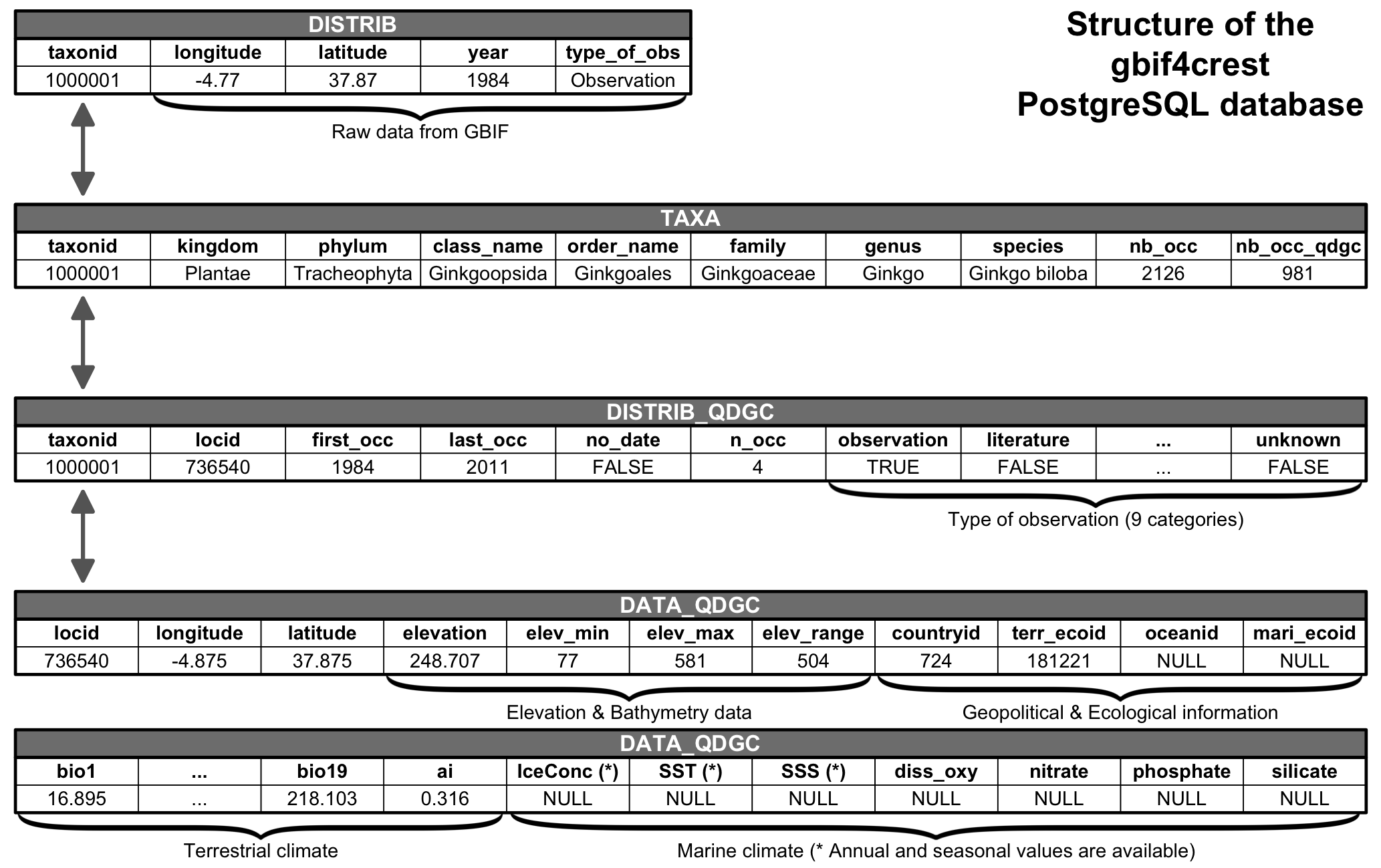
FiG. 2 Structure of the gbif4crest PostgreSQL database. By default, the package extracts data from the TAXA, DISTRIB-QDGC and DATA-QDGC tables. The DISTRIB table contains the raw occurrence data and can be used to process the data at a different spatial resolution for example.

Due to its large size, this database is not downloaded when installing the package, but it can be downloaded as a SQLite3 file format from here. No a priori SQL knowledge is required to use the database, so that users can benefit from the package’s interface to automatically query the database simply by providing study-specific parameters, such as the name of the taxa or boundaries for the study area, to import all the necessary data in the correct format to the R environment. Alternatively, advanced users can also directly query the database to extract and curate data from the DISTRIB or DISTRIB_QDGC tables using the dbRequest() function, and subsequently associate these data with climate variables. Also check the “Using the gbif4crest database” page under the More section.

References

[1] Chevalier, M., 2019. Enabling possibilities to quantify past climate from fossil assemblages at a global scale. Global and Planetary Change, 175, pp. 27–35. doi:10.1016/j.earscirev.2020.103384.

[2] The Global Biodiversity Information Facility, 2024. Occurrence data downloaded on 25 August 2024. doi:10.15468/dl.ZGMNQ9.

[3] The Global Biodiversity Information Facility, 2024. Occurrence data downloaded on 25 August 2024. doi:10.15468/dl.Y9KPWC.

[4] The Global Biodiversity Information Facility, 2024. Occurrence data downloaded on 25 August 2024. doi:10.15468/dl.UK2XV6.

[5] The Global Biodiversity Information Facility, 2024. Occurrence data downloaded on 25 August 2024. doi:10.15468/dl.QWCS68.

[6] The Global Biodiversity Information Facility, 2024. Occurrence data downloaded on 25 August 2024. doi:10.15468/dl.Q8ZUHH.

[7] The Global Biodiversity Information Facility, 2024. Occurrence data downloaded on 25 August 2024. doi:10.15468/dl.NUQ5TN.

[8] The Global Biodiversity Information Facility, 2024. Occurrence data downloaded on 25 August 2024. doi:10.15468/dl.MPFC47.

[9] The Global Biodiversity Information Facility, 2024. Occurrence data downloaded on 25 August 2024. doi:10.15468/dl.68HQXG.

[10] The Global Biodiversity Information Facility, 2024. Occurrence data downloaded on 25 August 2024. doi:10.15468/dl.7BVEJK.

[11] Fick, S.E. and Hijmans, R.J., 2017, WorldClim 2: new 1-km spatial resolution climate surfaces for global land areas. International Journal of Climatology, 37, pp. 4302–4315. doi:10.1002/joc.5086.

[12] Zomer, R.J., Trabucco, A., Bossio, D.A. and Verchot, L. V., 2008, Climate change mitigation: A spatial analysis of global land suitability for clean development mechanism afforestation and reforestation. Agriculture, Ecosystems & Environment, 126, pp. 67–80. doi:10.1016/j.agee.2008.01.014.

[13] Locarnini, R.A., Mishonov, A.V., Baranova, O.K., Boyer, T.P., Zweng, M.M., Garcia, H.E., Reagan, J.R., Seidov, D., Weathers, K.W., Paver, C.R., Smolyar, I.V. and Others, 2019, World ocean atlas 2018, volume 1: Temperature. NOAA Atlas NESDIS 81, pp. 52pp. data access.

[14] Zweng, M.M., Seidov, D., Boyer, T.P., Locarnini, R.A., Garcia, H.E., Mishonov, A.V., Baranova, O.K., Weathers, K.W., Paver, C.R., Smolyar, I.V. and Others, 2018, World Ocean Atlas 2018, Volume 2: Salinity. NOAA Atlas NESDIS 82, pp. 50pp. data access.

[15] Garcia, H.E., Weathers, K.W., Paver, C.R., Smolyar, I.V., Boyer, T.P., Locarnini, R.A., Zweng, M.M., Mishonov, A.V., Baranova, O.K., Seidov, D. and Reagan, J.R., 2019, World Ocean Atlas 2018, Volume 3: Dissolved Oxygen, Apparent Oxygen Utilization, and Dissolved Oxygen Saturation.. NOAA Atlas NESDIS 83, pp. 38pp. data access.

[16] Garcia, H.E., Weathers, K.W., Paver, C.R., Smolyar, I.V., Boyer, T.P., Locarnini, R.A., Zweng, M.M., Mishonov, A.V., Baranova, O.K., Seidov, D., Reagan, J.R. and Others, 2019, World Ocean Atlas 2018. Vol. 4: Dissolved Inorganic Nutrients (phosphate, nitrate and nitrate+nitrite, silicate). NOAA Atlas NESDIS 84, pp. 35pp. data access.

[17] Reynolds, R.W., Smith, T.M., Liu, C., Chelton, D.B., Casey, K.S. and Schlax, M.G., 2007, Daily high-resolution-blended analyses for sea surface temperature. Journal of Climate, 20, pp. 5473–5496. doi:10.1175/2007JCLI1824.1.

[18] Amante, C. and Eakins, B.W., 2009, Etopo1 1 Arc-Minute Global Relief Model: Procedures, Data Sources and Analysis. NOAA Technical Memorandum NESDIS NGDC-24. National Geophysical Data Center, NOAA. doi:10.7289/V5C8276M.

[19] Olson, D.M., Dinerstein, E., Wikramanayake, E.D., Burgess, N.D., Powell, G.V.N., Underwood, E.C., D’amico, J.A., Itoua, I., Strand, H.E., Morrison, J.C., Loucks, C.J., Allnutt, T.F., Ricketts, T.H., Kura, Y., Lamoreux, J.F., Wettengel, W.W., Hedao, P. and Kassem, K.R., 2001, Terrestrial Ecoregions of the World: A New Map of Life on Earth: A new global map of terrestrial ecoregions provides an innovative tool for conserving biodiversity. BioScience, 51, pp. 933. doi:10.1641/0006-3568(2001)051[0933:TEOTWA]2.0.CO;2.

[20] Costello, M.J., Tsai, P., Wong, P.S., Cheung, A.K.L., Basher, Z. and Chaudhary, C., 2017, Marine biogeographic realms and species endemicity. Nature Communications, 8, pp. 1–9. doi:10.1038/s41467-017-01121-2.