Extracting the signal from the background

In the previous chapter, average pace turned out to oversimplify the data. A hill workout, a tempo session, and a long run could produce similar averages even though their structures and purposes were completely different.

The pace distributions also contained a long tail of high values—that is, slow running. Most of it came from the warm-ups and cool-downs surrounding the main workout. These phases matter physiologically, but they are background when the question is whether my running performance itself is improving. Their duration and pace vary between sessions, so I cannot treat them as a constant offset and subtract the same amount from every run.

Before comparing performance across runs, I therefore need to identify the workout portion of each activity. The objective of this chapter is to find a simple, defensible set of rules that gives every lap in a structured session one of three labels:

• warm_up;
• work;
• cool_down.

The work laps are those that will be analysed in the next chapters to make performance prediction.

Defining the problem

A classification problem, but not a machine-learning one

Each run is divided into laps, and each lap must be assigned to a predefined category. This sounds like a typical supervised-classification problem, but the apparent sample size is misleading. I have a few hundred laps, yet they come from only a small number of runs, and laps from the same run are not independent observations.

Warm-ups and cool-downs also vary from one session to another. A statistical classifier would have too few independent examples of that variation and could easily memorise these particular runs.

That is a classic route to overfitting: excellent predictions for the training data, with no reason to expect the same performance on new runs.

I therefore use a deterministic rule-based classifier. Its conditions come from the structure of the programme, the physiology of heart-rate response, and practical knowledge of my own pace. If those ingredients are sufficient, there is no need to estimate a more complex model from so little data.

Simplicity is a feature, not an embarrassment. With a small dataset, an explicit rule can be easier to inspect, explain, and improve than a fitted model. It also leads to a more useful discussion than “the model predicted it”.

A first glance at the data

My watch has already divided each activity into useful laps. It vibrates whenever the training programme asks me to change effort, and each change creates a new lap in Garmin’s data. Laps are not all the same. Some are defined by distance, others by time, and their targets vary.

That information is stored in a third table in garmin_activities.db: activity_laps. Its primary key is the combination of activity_id and lap, so every row describes one lap within one activity.

The fields that will be most useful for this classification are:

• lap, start_time, and stop_time, which locate the lap within the run;
• distance, elapsed_time, and moving_time, which describe its size;
• avg_hr and max_hr, which summarise heart rate;
• hrz_1_time to hrz_5_time, which record the time spent in each heart-rate zone.

Three activities (runs 1, 7, 14, 18, and 19) are deliberately easy and continuous Zone 2 runs. They have no faster work block to isolate: the complete run is the training. I retain them in the data, but mark them as zone_2 because they should not contribute to the later comparison with my target pace.

The remaining fourteen runs contain a distinct workout. All begin with a warm-up, while some end as soon as the work block finishes and therefore contain no explicit cool-down. That variation is useful: a good rule must be able to return no cool-down rather than force one at the end.

What I know about warm-ups and cool-downs

Supervised classifiers are normally fitted on a training set and evaluated on unseen observations. I am not estimating these thresholds with an optimiser; I am translating prior knowledge into code and checking whether the resulting labels agree with the sessions I performed.

That distinction matters. It means I can use ALL my existing data to assess the performance of the classifier, instead of sacrificing some to estimate such paramters. New types of sessions will still need to be inspected when they appear.

The parameters translate the structure of the programme into explicit limits.

• Warm-ups and cool-downs appear only at the activity boundaries, so I consider at most the first four or final three laps (maximum_warm_up_laps and maximum_cool_down_laps).
• The distance limits add a second positional check: a warm-up cannot extend beyond 2.5 km (maximum_warm_up_dist), and a cool-down must begin within 1.5 km of the finish (maximum_cool_down_dist). These limits come the program I’m using.
• Heart rate responds to effort with a delay. At the start, it can remain low during the first part of a hard lap, so I make the warm-up criterion deliberately strict: at least 95% of the lap must be in Zones 0, 1, or 2 (warm_up_low_zone_share_threshold). This reduces the risk of absorbing the first workout lap into the warm-up.
• The same lag works in reverse after the effort stops. Heart rate can remain elevated during a genuine cool-down, so the end threshold is lower: at least 50% of the lap in the low zones (cool_down_low_zone_share_threshold).
• Pace provides one final guardrail at the start. A lap faster than 5 min/km is clearly part of the workout, so only laps with pace >= warm_up_pace_threshold can be warm-ups. I do not apply this pace criterion to cool-downs.

A reproducible start

The code follows the project structure established earlier in the notebook. I define every threshold together near the top rather than hiding numbers inside the classification code. This makes the final rule easy to audit and sensitivity-test.

# ---- Ready the tools ----
library(dbplyr)
library(dplyr)
library(fs)
library(ggplot2)
library(hms)
library(tidyr)


# ---- Locate the headquarters ----
setwd(
    path(path_home(), "DataSharp", "enter-the-mind", "running")
)


# ---- Describe the project ----
dir_inputs  <- path("_inputs")
dir_outputs <- path("_outputs")

dir_out_datasets <- path(dir_outputs, "data")
dir_out_figures  <- path(dir_outputs, "figs")

dir_create(c(dir_outputs, dir_out_datasets, dir_out_figures))

file_labelled_laps <- path(
    dir_out_datasets,
    "running-laps-labelled.rds"
)


# ---- Define the classification rule ----
maximum_warm_up_laps      <- 4
maximum_warm_up_dist      <- 2.5
maximum_cool_down_laps    <- 3
maximum_cool_down_dist    <- 1.5
warm_up_pace_threshold    <- 5

warm_up_low_zone_share_threshold   <- 0.95
cool_down_low_zone_share_threshold <- 0.50


# ---- Open the database connection ----
con <- DBI::dbConnect(
    RSQLite::SQLite(),
    dbname = path(
        dir_inputs,
        "DBs",
        "garmin_activities.db"
    )
)

Loading the laps and locating their boundaries

I first identify the running activities that belong to the programme. I join those identifiers to activity_laps inside the database so that R collects only the relevant laps.

runs_db <-
    tbl(con, "activities") |>
        filter(
            sport == "running",
            start_time >= "2026-06-29"
        ) |>
        select(
            activity_id,
            activity_name = name,
            activity_start_time = start_time
        )

laps <-
    tbl(con, "activity_laps") |>
        inner_join(runs_db, by = "activity_id") |>
        collect() |>
        mutate(
            activity_date = as.Date(activity_start_time),
            activity_label = paste(activity_date, activity_name)
        ) |>
        group_by(activity_id) |>
        arrange(lap, .by_group = TRUE) |>
        mutate(
            distance_from_start = cumsum(distance),
            distance_from_end   = rev(cumsum(rev(distance)))
        ) |>
        ungroup()

Within each activity, I order the laps before calculating distance in both directions. distance_from_start is the total distance completed by the end of a lap. distance_from_end is the distance covered by that lap and every lap after it. Together, they let me apply comparable distance limits at either boundary.

Garmin sometimes gives different runs the same default name. I therefore combine the date and name into activity_label, which keeps those activities separate in plots.

In total, the dataset contains 303 laps from 19 runs. The number of rows is useful computationally, but the number of independent runs is the more honest description of how much classification evidence I have.

Turning time and distance into usable features

The heart-rate-zone fields and lap moving time are stored as clock values, which first need to be converted into seconds. Garmin reports time in Zones 1 to 5, but their sum can be shorter than the lap’s moving time. I interpret the positive remainder as Zone 0: time below the lower boundary of Zone 1. pmax() keeps that remainder at zero when tiny rounding differences make the five reported zones fractionally longer than the moving time.

With that assumption made explicit, I calculate two features that are easier to use:

• low_zone_share, the proportion of lap time spent in Zones 0, 1, and 2;
• pace, calculated from lap moving time and distance in minutes per kilometre.

Deriving pace is necessary because the corresponding Garmin lap field is missing for some activities. Calculating it from two populated source fields recovers a homogeneous value for every lap in this dataset.

time_to_seconds <- function(x) {
    as.numeric(hms::as_hms(x))
}

laps <-
    laps |>
        mutate(
            lap_duration_seconds = time_to_seconds(moving_time),
            zone_1_seconds = time_to_seconds(hrz_1_time),
            zone_2_seconds = time_to_seconds(hrz_2_time),
            zone_3_seconds = time_to_seconds(hrz_3_time),
            zone_4_seconds = time_to_seconds(hrz_4_time),
            zone_5_seconds = time_to_seconds(hrz_5_time),
            tot_zone1_5_seconds = rowSums(
                pick(zone_1_seconds:zone_5_seconds),
                na.rm = TRUE
            ),
            zone_0_seconds = pmax(
                lap_duration_seconds - tot_zone1_5_seconds,
                0
            ),
            low_zone_share = if_else(
                lap_duration_seconds > 0,
                (zone_0_seconds + zone_1_seconds + zone_2_seconds) / lap_duration_seconds,
                NA_real_
            ),
            pace = if_else(
                !is.na(distance) & distance > 0,
                time_to_seconds(moving_time) / 60 / distance,
                NA_real_
            )
        )

laps |>
    select(
        activity_id,
        lap,
        distance_from_start,
        distance_from_end,
        low_zone_share,
        pace
    )

## # A tibble: 303 × 6
##    activity_id   lap distance_from_start distance_from_end low_zone_share  pace
##    <chr>       <int>               <dbl>             <dbl>          <dbl> <dbl>
##  1 23419618478     0                1               7.52         1         6.79
##  2 23419618478     1                2               6.52         1         6.38
##  3 23419618478     2                3               5.52         1         6.47
##  4 23419618478     3                4               4.52         0.952     6.48
##  5 23419618478     4                5               3.52         0.781     6.31
##  6 23419618478     5                6               2.52         0.220     6.22
##  7 23419618478     6                7               1.52         0.000993  5.92
##  8 23419618478     7                7.5             0.525        0         6.11
##  9 23419618478     8                7.52            0.0246       0.107     5.35
## 10 23455199693     0                1               6.39         1         6.27
## # ℹ 293 more rows

Pace protects the warm-up boundary

Heart rate zones alone cannot distinguish every boundary lap. A hard workout lap may still have a low heart rate at its beginning while the cardiovascular response catches up.

Pace provides a useful guardrail for the warm-up. In this programme, an early lap faster than 5 minutes per kilometre is clearly part of the workout. Because a smaller pace value means a faster speed, a warm-up candidate must have pace >= 5. I do not apply this threshold to cool-downs: after the main effort, their classification relies on position, distance from the finish, and low-zone share.

The pace threshold is a veto, not a complete definition of a warm-up. A slow lap still has to satisfy the position, distance, heart-rate, and continuity conditions.

The final classifier combines four conditions:

1. a warm-up can only occur among the first four laps and within 2.5 km of the start, while a cool-down must be among the final three laps and within 1.5 km of the finish;
2. a warm-up candidate must be no faster than 5 minutes per kilometre; cool-downs have no pace threshold;
3. the low-zone share must reach at least 95% at the beginning or 50% at the end;
4. warm-ups and cool-downs must form continuous sequences from their respective boundaries.

The continuity condition matters. An easy recovery lap in the middle of a hill or interval session must remain part of the workout, and a final lap that fails the cool-down heart-rate criterion must prevent earlier laps from being treated as a cool-down separated from the finish.

warm_up_laps <-
    laps |>
        filter(distance_from_start <= maximum_warm_up_dist) |>
            transmute(
                activity_id,
                lap,
                is_within_warm_up_distance = TRUE
            )

cool_down_laps <-
    laps |>
        filter(distance_from_end <= maximum_cool_down_dist) |>
            transmute(
                activity_id,
                lap,
                is_within_cool_down_distance = TRUE
            )

laps_labelled <-
    laps |>
        left_join(
            warm_up_laps,
            by = c("activity_id", "lap")
        ) |>
        left_join(
            cool_down_laps ,
            by = c("activity_id", "lap")
        ) |>
        group_by(activity_id) |>
        arrange(lap, .by_group = TRUE) |>
        mutate(
            lap_position = row_number(),
            laps_from_end = n() - row_number() + 1L,
            is_within_warm_up_distance = replace_na(
                is_within_warm_up_distance,
                FALSE
            ),
            is_within_cool_down_distance = replace_na(
                is_within_cool_down_distance,
                FALSE
            ),
            is_slow_enough_for_warm_up = replace_na(
                pace >= warm_up_pace_threshold,
                FALSE
            ),
            is_warm_up_candidate = replace_na(
                is_within_warm_up_distance &
                    is_slow_enough_for_warm_up &
                    low_zone_share >= warm_up_low_zone_share_threshold,
                FALSE
            ),
            is_cool_down_candidate = replace_na(
                is_within_cool_down_distance &
                    low_zone_share >= cool_down_low_zone_share_threshold,
                FALSE
            ),
            is_warm_up =
                lap_position <= maximum_warm_up_laps &
                cumall(is_warm_up_candidate),
            is_cool_down =
                laps_from_end <= maximum_cool_down_laps &
                rev(cumall(rev(is_cool_down_candidate))),
            segment_role = case_when(
                activity_id %in% c(23419618478, 23666794029, 23964251201, 24124614928, 24169121176) ~ "zone_2",
                is_warm_up   ~ "warm_up",
                is_cool_down ~ "cool_down",
                TRUE         ~ "work"
            )
        ) |>
        ungroup()

Building lookup tables with transmute()

The filtered warm_up_laps and cool_down_laps tables still contain every original lap column, but the joins need only the two columns forming the lap identifier—activity_id and lap—plus a new logical flag. transmute() creates those compact lookup tables:

warm_up_laps |>
    transmute(
        activity_id,
        lap,
        is_within_warm_up_distance = TRUE
    )

## # A tibble: 63 × 3
##    activity_id   lap is_within_warm_up_distance
##    <chr>       <int> <lgl>                     
##  1 23419618478     0 TRUE                      
##  2 23419618478     1 TRUE                      
##  3 23455199693     0 TRUE                      
##  4 23455199693     1 TRUE                      
##  5 23455199693     2 TRUE                      
##  6 23455199693     3 TRUE                      
##  7 23455199693     4 TRUE                      
##  8 23455199693     5 TRUE                      
##  9 23455199693     6 TRUE                      
## 10 23455199693     7 TRUE                      
## # ℹ 53 more rows

This is similar to mutate(), except that transmute() retains only the columns explicitly included or created—in effect, a mutate() followed by a select(). The subsequent left_join() attaches the flag to the complete laps table using the composite lap identifier. Laps absent from the lookup table receive NA, which replace_na() converts to FALSE.

Enforcing continuity with cumall()

The candidate flags assess laps individually, but a warm-up must be an unbroken sequence from the start. cumall() applies all() cumulatively:

is_warm_up_candidate  # TRUE TRUE FALSE TRUE
cumall(is_warm_up_candidate)
# TRUE TRUE FALSE FALSE

Once a lap fails, every subsequent result remains FALSE. A later easy lap therefore cannot re-enter the warm-up after the workout has started.

Cool-downs require the same operation from the finish rather than the start. I reverse the candidate vector, apply cumall(), and reverse the result back into lap order:

rev(cumall(rev(is_cool_down_candidate)))

Together, the lookup flags define where a boundary lap is possible, while the cumulative checks ensure that the final warm-up and cool-down labels remain continuous.

The result

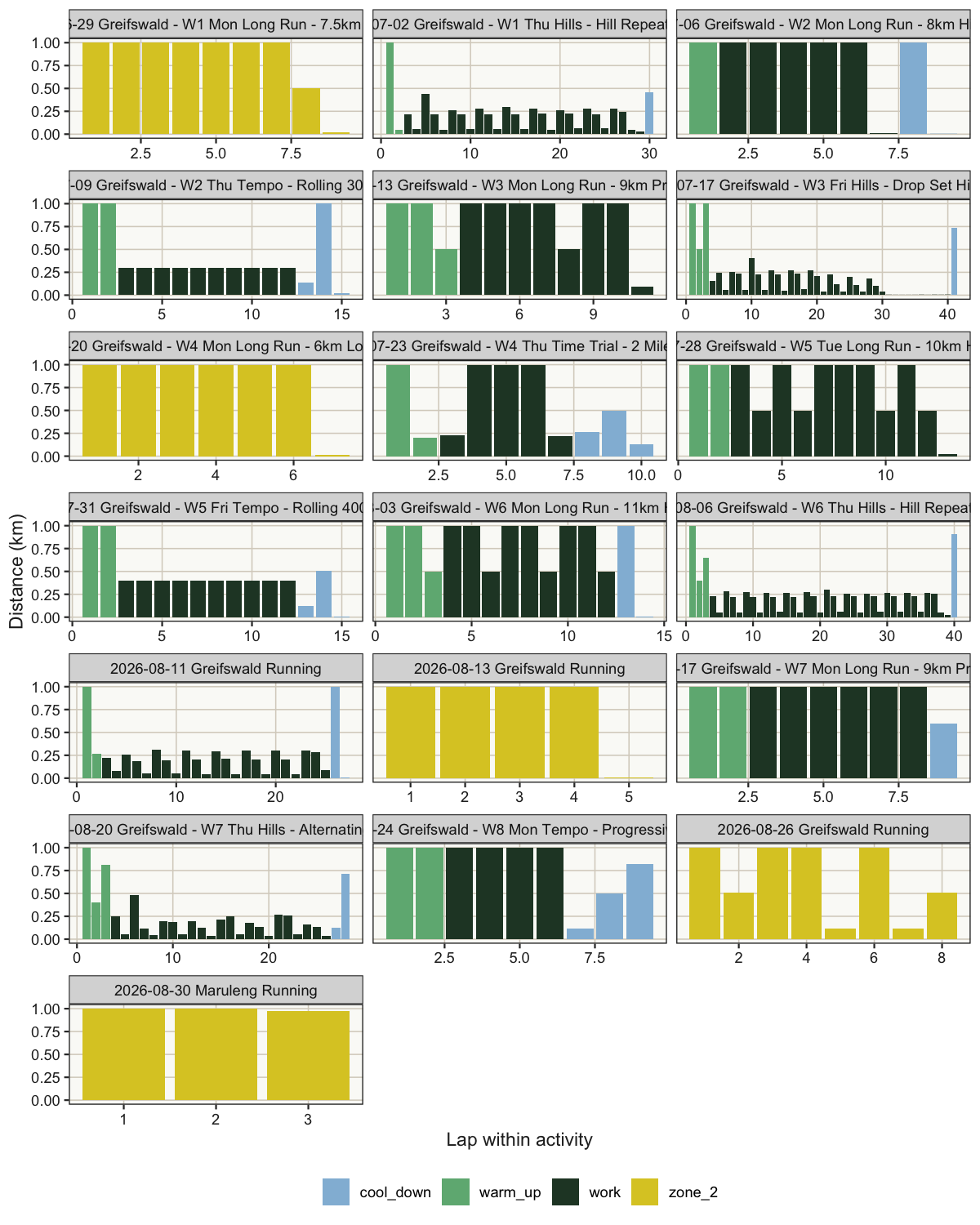
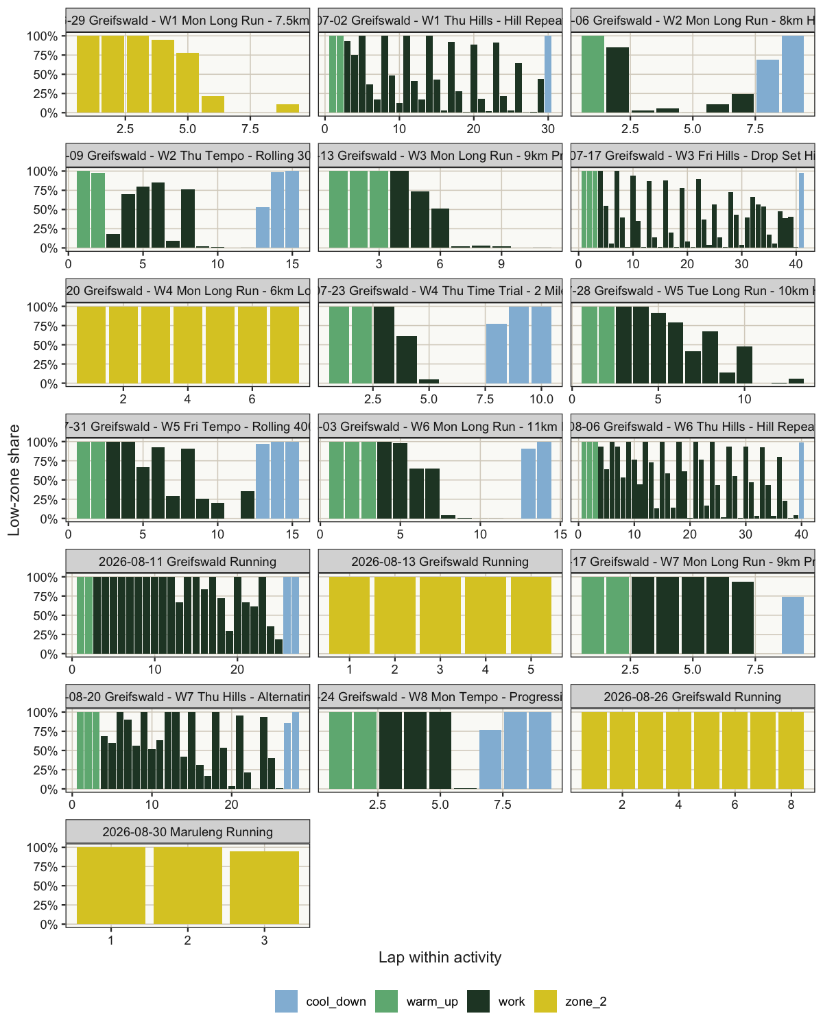
I can now inspect every result rather than relying on a single accuracy number. The three plots show the same labels against lap distance, low-zone share, and pace. Together, they reveal whether the rule has placed a boundary in a physically plausible location and why each lap received its category.

laps_labelled |>
    ggplot(
        aes(
            x = lap_position,
            y = distance,
            fill = segment_role
        )
    ) +
        geom_col() +
        facet_wrap(vars(activity_label), ncol = 3, scales = "free_x") +
        coord_cartesian(ylim = c(0, 1)) +
        labs(
            x = "Lap within activity",
            y = "Distance (km)",
            fill = "Classification"
        )

laps_labelled |>
    ggplot(
        aes(
            x = lap_position,
            y = low_zone_share,
            fill = segment_role
        )
    ) +
        geom_col() +
        facet_wrap(vars(activity_label), ncol = 3, scales = "free_x") +
        scale_y_continuous(
            limits = c(0, 1),
            labels = scales::label_percent()
        ) +
        labs(
            x = "Lap within activity",
            y = "Low-zone share",
            fill = "Classification"
        )

laps_labelled |> select(start_time, lap, low_zone_share, segment_role) |> filter(start_time>="2026-08-17")#

## # A tibble: 57 × 4
##    start_time                   lap low_zone_share segment_role
##    <chr>                      <int>          <dbl> <chr>       
##  1 2026-08-17 17:10:27.000000     0          1     warm_up     
##  2 2026-08-17 17:16:22.000000     1          1     warm_up     
##  3 2026-08-17 17:22:03.000000     2          1     work        
##  4 2026-08-17 17:27:50.000000     3          1     work        
##  5 2026-08-17 17:33:33.000000     4          1     work        
##  6 2026-08-17 17:39:08.000000     5          1     work        
##  7 2026-08-17 17:44:38.000000     6          0.935 work        
##  8 2026-08-17 17:50:00.000000     7          0     work        
##  9 2026-08-17 17:54:55.000000     8          0.736 cool_down   
## 10 2026-08-20 16:32:35.000000     0          1     warm_up     
## # ℹ 47 more rows

laps_labelled |>
    ggplot(
        aes(
            x = lap_position,
            y = pace,
            fill = segment_role
        )
    ) +
        geom_col() +
        facet_wrap(vars(activity_label), ncol = 3, scales = "free_x") +
        scale_y_continuous(
            limits = c(0, 12)
        ) +
        labs(
            x = "Lap within activity",
            y = "Pace (min/km)",
            fill = "Classification"
        )

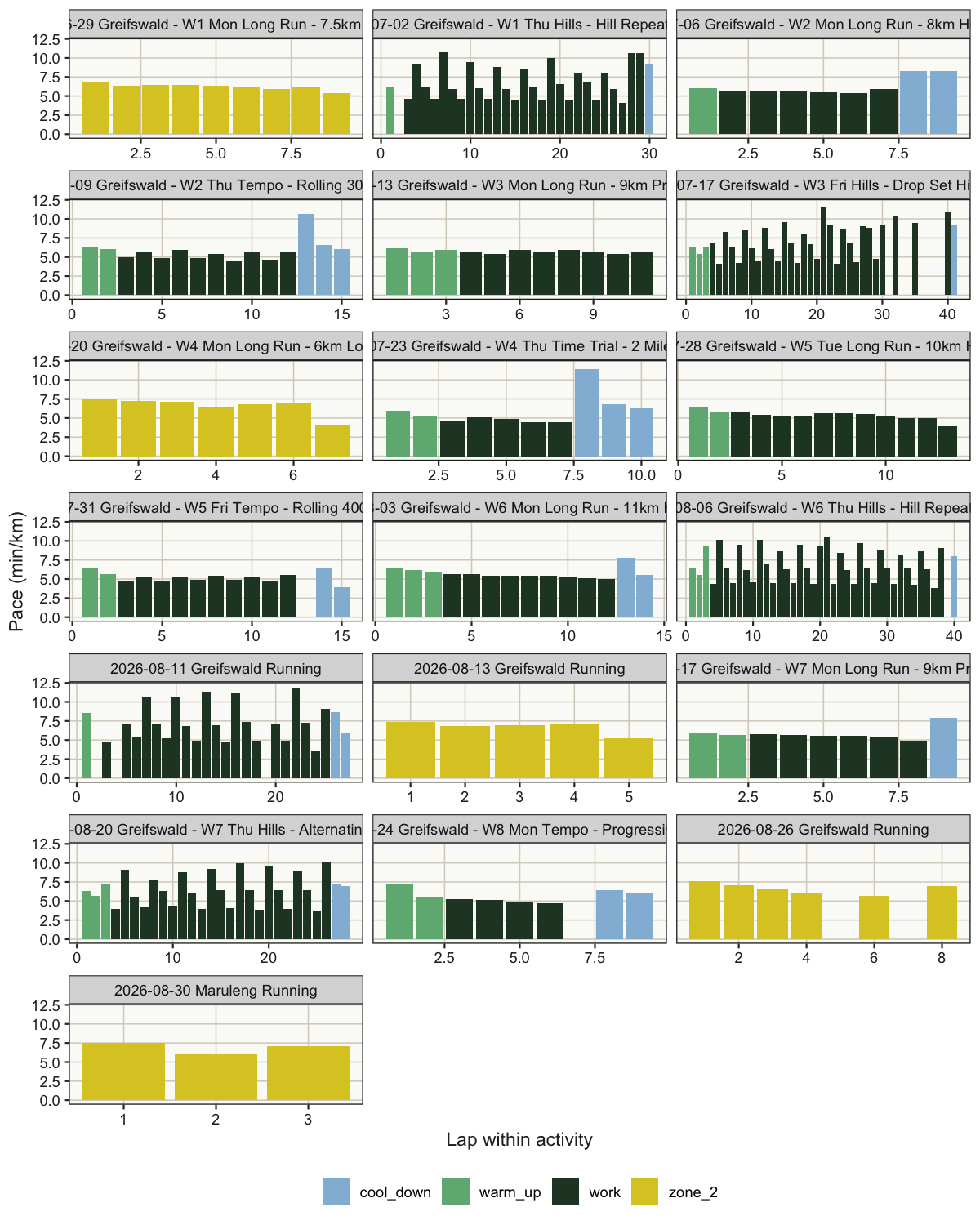
For the fourteen sessions containing a distinct workout, the automatic labels match the intended structure lap for lap. I find no false warm-ups, false cool-downs, or missed boundary laps in the current data. Within its intended scope, the rule therefore achieves a perfect classification on this snapshot.

The result shows that the chosen constraints are sufficient for the sessions observed so far; it does not guarantee that a new session structure will behave identically. The advantage of the rule is that any future failure will be visible and each decision can be traced back to an explicit condition.

When there is no background to remove

As established at the beginning of the chapter, Zone 2 runs do not have the three-part structure this rule is designed to find. Runs 1, 7, and 14 were easy and continuous from beginning to end, without a distinct warm-up, harder workout, and cool-down.

These are not three additional classification errors. They are activities outside the scope of the boundary rule. I identify them from the training programme and assign the whole activity to zone_2 before the labels are used downstream. This is an activity-level scope decision, not a threshold tuned to make individual laps look correct.

The recovery runs remain in the labelled data because they are real and valuable training. They simply answer a different question. When I later calculate performance against my pace target, zone_2 activities can be excluded without discarding them or pretending that they contain transitions that never occurred.

This distinction matters: a classifier can perform well on the cases it was designed for while still being inappropriate for a different kind of observation. The solution is to define the scope of the rule, not to call every out-of-scope case a threshold error.

Saving the classified laps

This is the natural stopping point for the chapter. laps_labelled contains the original lap fields, the derived distance, heart-rate, and pace features, and the final classification. I save that complete table rather than immediately returning to the more detailed activity records.

An RDS file preserves R’s column types and lets the next chapter restart with a single readRDS() call.

saveRDS(laps_labelled, file_labelled_laps)

DBI::dbDisconnect(con)

Take-home message

The chapter produces one reusable restart point: running-laps-labelled.rds. It preserves every lap, the derived features, and the evidence behind each classification without discarding any source data.

The simple rule perfectly reproduces the intended lap structure of the fourteen observed workouts. It does so without fitting a statistical model: the parameters express where a boundary can occur, how heart rate behaves around effort, and what pace is unmistakably part of the workout. The three Zone 2 runs are separated by design because no background should be removed from them.

A perfect result on the current runs is not the same as a universally perfect classifier. It is evidence that these transparent, out-of-the-box constraints are adequate for the data and programme so far. That is enough for the next stage, while keeping the assumptions visible if a future run breaks them.

What’s next

I have extracted the signal from its background, but a hill session is still not directly comparable with a tempo run or a long run. In the next chapter, I will ask the same standardised question of every eligible activity: What five-mile performance does this run represent?